Over the last couple of decades, the lattice Boltzmann method (LBM) has grown into a potent alternative methodology for computational fluid dynamics (CFD). As such, CFD has been traditionally developed using the Navier-Stokes equations as a starting point. But there are several advantages to using the LBM, chiefly the extreme simplicity of the approach (easy coding) and the inherently parallel nature of the computations (scales easily to large machines). The LBM is akin to an explicit numerical scheme, in that the variable at the new time level can be calculated based on the (local) values of the variable at the previous time level.
Unlike regular CFD, where the primary dependent variables are the velocity components, the density and the pressure, the LBM works with particle velocity distribution functions, or PDFs. A simplified way of understanding the LBM is to imagine that there are a set of discrete points in space (lattice points) and there is a set of finite directions at each lattice point along which fluid particles can move or “stream”. During each time step, particles “stream” or hop from one lattice point to another along these finite directions and then “collide” with each other, conserving mass and momentum. This collision event leads to a new distribution of particles, which then streams again to neighboring lattice points. For more information about the LBM, you can refer to several excellent review articles available on the internet.
A simple application of the LBM is to solve for two-dimensional flow inside a square cavity. In this problem, the square cavity is completely filled with a constant viscosity fluid. The three side walls of the cavity are fixed and the top wall suddenly starts moving to the right with a constant velocity, dragging the adjacent fluid along with it and causing a re-circulating flow to develop inside the cavity. In this blog, we will provide a canonical LBM implementation of this problem (for low Reynolds numbers) and provide detailed CPU and GPU versions of the code so interested users can see for themselves how easy it is to migrate from the C++ (CPU version) to the CUDA (GPU version) and the amazing speed-up than can result from doing so.
The CPU approach
A simple LBM code that can be implemented on the CPU can be obtained by following the link below. This 2D implementation uses the D2Q9 model, which means we have a 2 dimensional model with 9 discrete velocity directions.
Click here to download the CPU code
The CPU version sweeps through each lattice point in a sequential manner and finds the new distribution functions after streaming and collision at that lattice point. However, all of these updates are completely independent of each other and they can be performed in parallel.
The GPU approach
The basic idea behind this particular GPU implementation is very simple. We allocate and initialize all the relevant arrays directly on the GPU. Once this is done (we will assume that we have enough memory to accomplish this task), the actual updating of the PDFs because of streaming and collision is performed in parallel using thousands of threads that each work on independent lattice points. The complete CUDA code for implementing this idea is provided below for reference. As we said, this is just a demonstration of how to port the CPU based C++ code to the GPU and we do not wish to imply that this is the best and most efficient implementation of the LBM on the GPU. But a code is worth a thousand words:
Click here to download the GPU code
The initial part of the code starts off on the CPU and allocates space to store the PDF arrays on the GPU using cudaMalloc. After this, the main portion of the algorithm runs completely on the GPU. The only instance where we would be required to move data from the GPU to the CPU is when we want to write it to output files for post-processing purposes. This is not done in this example for clarity and conciseness.
RESULTS
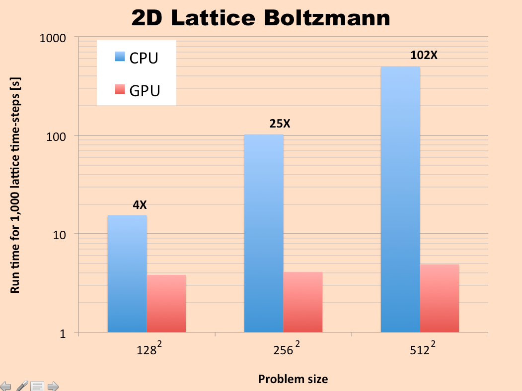
We ran this problem using both the CPU version and the GPU version for a range of grid sizes, starting from a 128 x 128 lattice and going up to a 512 x 512 lattice. The results for total simulation time are summarized in the graph below. It can be observed that the GPU version completely outperforms the CPU version, even for the 128 x 128 grid.