Laplace’s equation is one of the simplest possible partial differential equations to solve numerically. It applies to various physical processes like electric potentials and temperature fields. In this blog, I will highlight a simple numerical scheme to solve this equation referred to as Jacobi iteration. Starting with a simple CPU based C++ code, I will highlight how easy it is to port this code to the GPU using CUDA.
We’ll focus on a particular example from heat transfer, where the goal is to solve for the steady-state temperature field T(x,y) and the solution domain is a square of size L in the X-Y plane. The boundary conditions are as follows:
- Left edge: x = 0, T(0, y) = 1
- Right edge: x = L, T(L, y) = 0
- Bottom edge: y = 0, T(x,0) = 0
- Top edge: y = L, T(x,L) = 0
Without going into too many details, the core algorithm for solving the temperature field inside the domain boils down to this simple equation:
T(i,j) = 0.25 * [T(i-1,j) + T(i+1,j) + T(i,j-1) + T(i,j+1)] ——- (1)
Here, it is assumed that the square domain is represented using a computational grid of N x N points, equally spaced along X and Y. Equation (1) essentially states that the temperature value at any node point equals the arithmetic average of the 4 neighboring temperature values. The value at the boundary node points are known from the boundary conditions and the objective is to iteratively find the interior T(i,j) values using Eq.(1).
The CPU approach
We define two 2D arrays, T(1:N,1:N) and T_new(1:N,1:N) and essentially loop over all interior node points in the domain, updating T_new(i,j) at each interior node point using values from T(i,j) from the previous iteration. The core Jacobi function from the CPU code is copied below for reference.
void Jacobi(float* T, float* T_new)
{
    const int MAX_ITER = 1000;
    int iter = 0;

    while(iter < MAX_ITER)
    {
        for(int i=1; i<NX-1; i++)
        {
            for(int j=1; j<NY-1; j++)
            {
                float T_E = T[(i+1) + NX*j];
                float T_W = T[(i-1) + NX*j];
                float T_N = T[i + NX*(j+1)];
                float T_S = T[i + NX*(j-1)];
                T_new[i+NX*j] = 0.25*(T_E + T_W + T_N + T_S);
            }
        }

        for(int i=1; i<NX-1; i++)
        {
            for(int j=1; j<NY-1; j++)
            {
                float T_E = T_new[(i+1) + NX*j];
                float T_W = T_new[(i-1) + NX*j];
                float T_N = T_new[i + NX*(j+1)];
                float T_S = T_new[i + NX*(j-1)];
                T[i+NX*j] = 0.25*(T_E + T_W + T_N + T_S);
            }
        }
        iter+=2;
    }
}
In this implementation, we update T_new(i,j) using values from T(i,j) and then update T(i,j) using values from T_new(i,j). This essentially completes two Jacobi iterations. We keep going until a set number of maximum iterations is reached (1,000 in the above code snippet). The CPU implementation is slow mainly because we update points in a sequential fashion, one after the other. But this was pretty much the best you could hope for before parallel computing.
The GPU approach: CUDA
Notice that each update of T_new(i,j) in the above code is independent of every other update. So what if we could update all node points in parallel at the same time? This is exactly what we do using GPUs.
Click here to download the GPU (CUDA) code
Notice that the basic instruction for updating the node point using the average of its neighbors is identical in the GPU code. However, the loop over i and j has disappeared in the kernel (function running on the GPU). The key point to understand is that this kernel is executed in parallel using several threads on the GPU using the triple chevron notation <<< >>>.
Each thread figures out which node point it is updating and updates the value in the appropriate memory location. When all threads are done updating their node point, we move on to the next iteration. Obviously, the GPU approach is faster than the CPU approach, but there is also some time spent in allocating resources on the GPU and in copying data from the CPU to the GPU. Thus, the speed up in the actual execution of the Jacobi iteration may not become apparent until the mesh size is large.
RESULTS
In the figure below, a comparison of the run-time between the CPU and the GPU is attached. For the largest grid shown below, we obtained a speed up of 143X for the CUDA version compared to the CPU code.
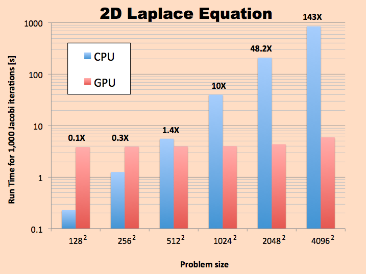
It will be apparent that the GPU version using CUDA is way faster than the CPU version for mesh sizes larger than 256 x 256. In reality, as mentioned above, the actual Jacobi iteration (or convolution) part is always faster than the CPU version.
To conclude, this example illustrated how a simple partial differential equation (PDE) can be solved on the GPU provided we can execute it as a “single instruction on multiple data” (SIMD) algorithm. The basic idea of creating a workspace (array) on the GPU and updating elements of this array in parallel can be applied even to more complex PDEs and algorithms, provided they can be written in a SIMD fashion. The only limitation in this approach is the amount of memory available on the GPU.