Category Archives: R programming language

The world of R: drawing y = f(x) using “curve”

In this post, we continue learning about the R programming interface. Making simple X-Y plots using a mathematical expression of the type

y = f(x)

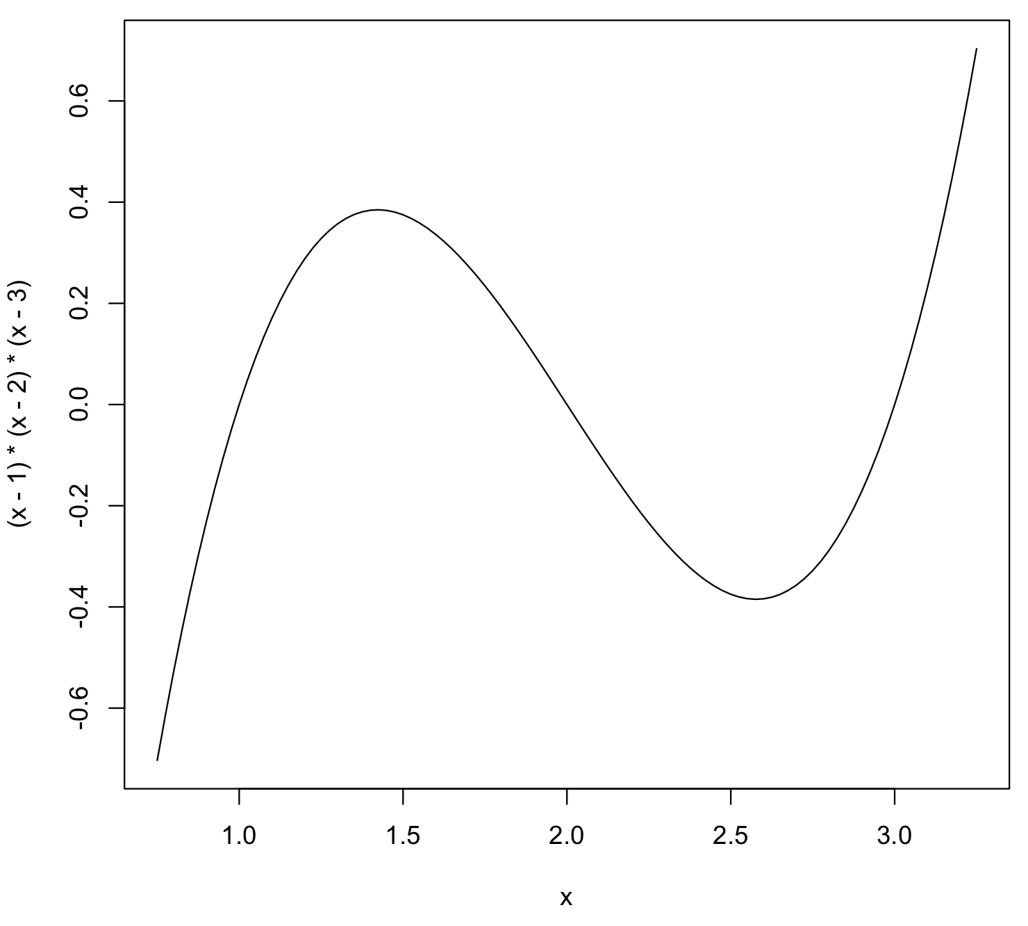
is a nice way to learn how functions behave and for finding out the roots of polynomial functions. In R, the curve command can handle almost anything you wish to plot and analyze. Let’s assume that you have a function of the form:

y = (x – 1)(x – 2)(x – 3)

In this case, we already know that the roots of this function [x values where y = f(x) = 0] are x = 1, x = 2 and x = 3. Thus, picking a range of x-values over which this function shows some interesting behavior is easy. Let’s pick the range from x = 0.75 to x = 3.25.

This is how you would plot this function in the X-Y plane using R:

curve((x-1)*(x-2)*(x-3),from=0.75,to=3.25)

functionPlot001

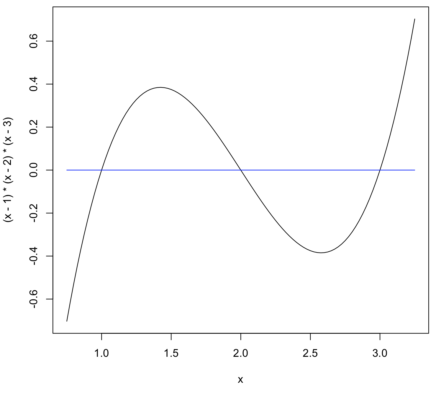
To overlay another plot on the same window, use “add = TRUE” as an additional parameter to the curve command. For example, to insert a blue-colored horizontal line (y = 0) in the above plot, use:

> curve(0*x,from=0.75,to=3.25,col='blue',add=TRUE)

functionPlot002

You can control the number of points “n” used to draw the curve (default n = 101), add custom labels for the axes and draw logarithmic plots. Consult this link  for additional details about all the parameters we can use for the curve command.

Falling in love with R

I had heard about this amazing language for statistical analysis and finally decided to give it a shot after reading a sample first chapter preview from “R in Action” by Robert Kabacoff (this looks like a great book by the way and is on my list of books to buy). The first thing was to download and install the software on my Mac, which was a quick and entirely painless process. You fire up R by clicking on the “R” icon in the Mac applications folder.

The initial window looks pretty much like a unix terminal. To see what R can do, I decided to start with a simple linear regression example. The set of R statements below create a series of (x,y) coordinates and then plot each point on a simple plot.

> x <- c(0,1,2,3,4,5,6,7,8,9,10)
> y <- c(0,1,2,2,4,4,5,6,7,10,11)
> plot(x,y)

Here is the result:

R_y_vs_x

Next, we create a least-squares fit to the data and plot the resulting line on top of the data:

> model <- lm(y~x)
> yfit <- model$fitted.values
> lines(x,yfit)

And this is what we get:

R_least_squares_fit

You want the actual equation of the line? The slope and Y-intercept can be obtained using:

> lm(y~x)

Call:
lm(formula = y ~ x)

Coefficients:
(Intercept)            x  
     -0.500        1.045

Now this was a really simple example, but it was enough to illustrate what R can do. And going by first impressions, it looks like I will be exploring a lot of R in the future.